Research Multiphase and index-matched flows

Tomo-PTV of buoyancy driven spheres

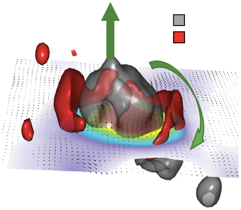
A small acrylic ball rises through a tank of salt water. It zigzags, speeds up, slows down, and leaves a trail of vortices behind it. We wanted to measure the forces that make it do that, on a body that is completely free to move. To get there, we first had to make the sphere disappear, and then invent a way to find it again.

Based on two papers from the lab, published in the International Journal of Multiphase Flow (2026) and Measurement Science and Technology (2026). Links at the end.

The octagonal tank, 70 cm tall, with four Phantom v2640 high-speed cameras looking in.

The experiment in four numbers

4high-speed cameras, recording 4,800 frames every second

100,000fluorescent tracer particles, each smaller than a hair's width

1.489refractive index of both the acrylic sphere and the salt solution

1%of a diameter: how precisely we locate a sphere we cannot see

Why this matters

Almost anything that rises or sinks through a liquid is steered by the wake it leaves behind. The same coupling turns up wherever industry moves one phase through another.

Solids settling in a thickening tank

How quickly a suspension clears depends on how its particles fall, and falling particles rarely travel in straight lines.

Bubbles and agglomerates in reactors

In a chemical reactor, how long a bubble or a clump stays in the vessel helps set how much of it has time to react.

Oil droplets rising from a well

Droplets escaping an underwater well spread through the water column along the wandering paths their own wakes give them.

Why chase a rising ball?

Simulations have described the zigzag for years; nobody had measured the forces on a freely moving sphere while watching the wake that causes them.

A sphere rising through a liquid is one of the oldest problems in fluid mechanics and still not a solved one. Seeds falling from a tree, bubbles in a reactor, sediment settling in a tank, oil droplets escaping from a well: all of them are bodies moving freely through a fluid, pushed around by the very wake they create.

The wake is the trouble. As the sphere moves, it sheds vortices, and each vortex tugs on the sphere. The result is a path that wobbles, zigzags or spirals. Simulations have described this dance for years, but nobody had directly measured the forces on a freely moving sphere while watching the wake that causes them. Most experiments held the sphere still or on a tether. We wanted to let it go.

Six wandering three-dimensional paths measured for rising spheres of three sizes — Six measured paths of spheres between 7.9 and 11.1 mm across, released at the bottom of the tank and tracked as they rose. None of them goes straight up: this wandering is what the rest of the page sets out to explain.

Step one: make the sphere disappear

Match the refractive index of the sphere to the liquid and it vanishes; make the tracers fluorescent and even its reflections go.

To see the flow around a moving body in three dimensions, we light up tiny tracer particles with a laser and film them from four angles at once. Light bends when it passes from water into acrylic, so a plain acrylic sphere would distort everything behind it, exactly where we want to look.

The cure is an old trick with a modern twist. A concentrated solution of sodium iodide, about 62% salt by weight, has the same refractive index as acrylic, so light travels straight through the sphere as if it were not there. We then make the tracers fluorescent and put filters on the cameras that block the laser's own colour, which removes the last faint reflections from the sphere's surface. The recordings become pristine. They also lose the sphere entirely.

For the specialist

Working fluid 62 wt% NaI, density 1820 kg/m³, kinematic viscosity 1.1 × 10⁻⁶ m²/s, refractive index 1.489. Tracers: Rhodamine-B-coated PMMA, 1–20 µm, imaged through 550 nm long-pass filters. Acrylic spheres of 6.35–12.7 mm and density ratio m* = 0.65, released from a 400 mm pipe so they reach terminal velocity before entering the 110 × 75 × 25 mm measurement volume. Re_T = 1500–3500, Ga = 848–2397. Tracks from Shake-The-Box, Eulerian fields by VIC#, pressure by GPU Omni3D integration.

An acrylic sphere sitting half in air and half in salt solution: the upper half is clearly visible, the submerged half has vanished — Index matching, demonstrated in one photograph: a single acrylic sphere held half in air and half in the sodium iodide solution. The half above the surface is obvious; the submerged half has disappeared.

Camera image with ordinary tracers: the sphere glows as a bright disc — What one camera actually records. Left, with ordinary tracers, the sphere lights up and swamps the particles around it. Right, with fluorescent tracers behind a filter, nothing is left but particles. The dotted circle was drawn in afterwards to show where the sphere was.

Camera image with fluorescent tracers and a filter: only a faint dotted outline marks where the sphere is — What one camera actually records. Left, with ordinary tracers, the sphere lights up and swamps the particles around it. Right, with fluorescent tracers behind a filter, nothing is left but particles. The dotted circle was drawn in afterwards to show where the sphere was.

Step two: find it anyway

An invisible sphere still leaves three fingerprints in the flow, and together they pin it down to about one percent of its diameter.

An invisible sphere still leaves fingerprints in the flow, and three of them are enough to pin it down. There are no tracers inside it, so it shows up as a hole in the particle cloud. It shoves fluid upward just ahead of itself, and by conservation of mass the fluid a little farther out must come back down. And the fluid inside it does not spin, while the wake behind it is full of vortices.

We turn the three fingerprints into a single score for every candidate position and let an optimizer slide toward the best one, frame after frame, starting each search where the sphere was a moment ago. The result is a position known to about one percent of the sphere's diameter, without a single marker on the sphere itself, so its surface, and its physics, stay untouched.

For the specialist

The cost function J(x) = D(x) + w₁[−V_inner + V_outer] + w₂[Q_inner − Q_outer] combines normalised tracer density in a sphere of radius R, mean vertical velocity in the upper hemisphere within 1.1R against a shell between 1.5R and 2R, and mean Q-criterion inside against a shell out to 2.5R. It is minimised by Polak–Ribière conjugate gradients with a backtracking line search. Weights w₁ = 3.08 and w₂ = 4.42 were calibrated for stable, jitter-free convergence. Positional uncertainty from the Hessian of J at the minimum: mean 0.7–1.2% d, worst case below 0.08 d; robust to ±10% weight changes, 25% search-radius changes and 10% added noise.

A dense cloud of reconstructed tracer positions with an empty rounded region where the sphere is — **Fingerprint one: a hole.** The measured cloud of tracer particles. No tracers can sit inside the sphere, so it appears as an empty pocket in an otherwise dense cloud.

Stacked horizontal slices of vertical velocity showing a ring-shaped pattern around the sphere's position — **Fingerprint two: a ring.** Vertical velocity on stacked horizontal slices. The sphere pushes fluid up just ahead of itself and that fluid must return downward farther out, leaving a ring centred on the sphere.

Surfaces of equal swirl in the wake, drawn over a slice of the measured velocity field with its vectors — **Fingerprint three: swirl, but only behind.** Surfaces of equal swirl over the measured velocity field. Vortices crowd the wake and never appear inside the body, so the contrast between the two locates it.

Three-dimensional rendering of the flow around the rising sphere, with upward-moving fluid in grey and downwash in red — The same flow in three dimensions, seen from the sphere: the fluid it pushes up ahead of itself (grey) and the downwash that returns beside it (red).

What the sphere feels

Drag stays high while the vortex threads cling to the sphere and collapses the moment they let go, and that release is what sets up the next zigzag.

With the position known, the measured velocity field gives us the pressure everywhere, and the pressure on the sphere's surface gives us the force. For the first time, drag and lift on a freely moving sphere can be followed through time, together with the wake that produces them. Here is half an oscillation of the 11.11 mm sphere, about a fifth of a second, from A to J.

Five snapshots of the sphere and its wake, labelled A to E, showing two twisted vortex threads growing behind the sphere — Half an oscillation of the 11.11 mm sphere, read left to right: snapshots A to E on the top row, F to J below, with the elapsed time printed under each. The sphere is the black disc; the red shapes are vortices in its wake, drawn as surfaces of equal swirl (Q = 1800 s⁻²). Threads grow, cling, then pinch off into rings.

Five more snapshots, F to J, showing the vortex threads detaching and breaking into rings — Half an oscillation of the 11.11 mm sphere, read left to right: snapshots A to E on the top row, F to J below, with the elapsed time printed under each. The sphere is the black disc; the red shapes are vortices in its wake, drawn as surfaces of equal swirl (Q = 1800 s⁻²). Threads grow, cling, then pinch off into rings.

A to C. Two twisted threads of vorticity trail behind the sphere. As long as they stay attached and coherent, they pull on its rear, the drag is high, and the sphere slows down. Because the two threads are unequal, they also push it sideways.

D to G. The threads weaken and the suction eases. Drag falls to almost nothing and the sphere accelerates again, with a brief sideways wiggle as the loading becomes lopsided.

H to J. The threads let go completely and roll up into two vortex rings that drift away. Released from its wake, the sphere speeds up sharply, and a new thread begins to form on the other side. That is what will make the next half-cycle swing the other way: the zigzag.

For the specialist

Forces are obtained by integrating the reconstructed surface pressure, F = −∮ p n dS, so they represent the dynamic component only (buoyancy is not included). For the 11.11 mm sphere (Re_T ≈ 2880, m* = 0.65) the wake shows a primary and a secondary vortex ring per half-cycle, the asymmetric four-ring (4R) mode of Horowitz & Williamson (2010), with the sphere sitting near the 2R/4R boundary. The measured drag history is phase-locked to the attachment and pinch-off of the streamwise vortex threads; the transition from thread to rings at H–I is observed here for the first time as it happens.

The sphere drawn at seven positions along its rising path, each coloured by the pressure on its surface — The sphere drawn at seven moments along its path, each copy painted with the pressure (in pascals) on its own surface: high on the nose, low on the wake side, and visibly lopsided whenever a vortex pulls from one flank. Integrating this colour over the surface is what gives the force.

Time histories of the sphere's speed, drag and lift over 220 milliseconds, with the moments A to J marked — The forces, measured rather than modelled: speed (blue, left axis) with drag (dotted) and lift (dashed) in millinewtons on the right axis, over the same 220 ms. Every dip in speed lines up with a peak in drag, and the letters mark the ten snapshots above.

Size changes everything

Change nothing but the diameter and the wake switches character entirely, yet the same measurement method keeps working across all of it.

The three spheres are made of the same material in the same liquid; only their diameter differs, and with it the Reynolds number. That is enough to change the character of the motion. The 11.11 mm sphere sheds pairs of rings and wanders in three dimensions. The 9.53 and 7.93 mm spheres rise almost straight, shedding one symmetric ring at a time, and the smallest one is governed by vortices hugging its surface rather than by the larger structures in its wake.

Across all three, the pattern holds: bigger sphere, faster rise, larger swings in drag. It confirms that the invisible-sphere method produces forces that behave consistently across regimes, which is what makes it a measurement technique rather than a one-off.

For the specialist

Re_T ≈ 2880, 2170 and 1760 for d = 11.11, 9.53 and 7.93 mm. The two smaller spheres show the canonical two-ring (2R) regime: symmetric, periodic, phase-locked shedding with lift alternating about zero. |V₁₁| > |V₉| > |V₇| and F_d,11 > F_d,9 > F_d,7. Each recording covers roughly half a shedding cycle, a limit set by camera resolution rather than by the method.

Wake snapshots for the 9.53 mm sphere: a single compact vortex ring forming beneath it — The 9.53 mm sphere, in five consecutive snapshots from left to right. Instead of the twisted pair of threads the larger sphere trails, one compact ring forms beneath the body at a time, and the path stays almost straight.

Wake snapshots for the 7.93 mm sphere: vorticity stays close to the sphere's surface — The smallest sphere, 7.93 mm, over a comparable sequence. Here the vorticity stays close to the body itself and the far wake barely tugs on it, which is why this sphere rises the straightest of the three.

Step three: teach the reconstruction about the body

Standard reconstructions assume the whole volume is fluid; telling the solver where the solid is repairs the velocities exactly where the forces come from.

Tracking particles gives velocities at scattered points. To compute pressure, vorticity or forces, those points have to be turned into a smooth field on a regular grid, and every method for doing so assumed the whole volume is fluid. Around a moving body that assumption fails precisely where it matters most: the method happily invents velocity inside the solid and ignores the fact that fluid at the surface must move with the surface.

Our second paper fixes this. At every instant, each grid point is classified by its distance to the body: inside, on the thin shell around the surface, or in open fluid. The shell is forced to move with the body, incompressibility is imposed only in the fluid, and points the body has just vacated are told to forget their past. The whole thing is one solve, works for stationary walls, translating, rotating or several bodies alike, and switches itself off wherever there is no body at all.

For the specialist

LE-DM extends constrained cost minimisation (Agarwal et al. 2021) to a time-dependent fluid–solid partition defined by a signed-distance field φ(r, t). Shell nodes (0 ≤ φ ≤ Δ/2) and interior nodes carry Dirichlet constraints u = U_s + ω_s × (r − X_s); open-fluid nodes carry divergence constraints, with second-order one-sided stencils next to the interface. Data weights are damped near the surface according to the body-detection uncertainty σ_Γ; the temporal prior is reset at newly exposed nodes; a coverage-adaptive graph Laplacian regularises data-starved wake cells. The saddle-point system is solved with MINRES (≈4.5 s per snapshot for 221,000 unknowns on one CPU core). Analytical oscillating sphere: first-cell error 14% → 3% of U₀. CFD rising sphere: 1.5–3.5% full-domain error. Tumbling prolate spheroid: 4.6% full-domain, 2.4–3.4% near-surface. Code: github.com/TFMLTechnion/LEDM.

Three-panel schematic: the tracer volume with the moving body, the grid classified into solid, shell and fluid points with its stencils, and the resulting reconstructed velocity field — The method in one figure. (a) The measured tracer volume, with the body's shape and motion already known from the detection step. (b) A signed distance to the surface sorts every grid point into solid, shell or fluid, and decides which stencil is used near the boundary. (c) The reconstruction that follows: divergence-free in the fluid, pinned to the body's own motion at the shell, and corrected in the region the body has just left.

Four reconstructions of the same measurement side by side; only the second leaves the sphere's interior blank — The same experimental snapshot reconstructed four ways. Only the masked method (second panel) knows there is a sphere there; the others paint velocity straight through the solid, and the last one leaves more than half of the wake empty.

Reconstructed speed at the sphere's surface over time for four methods; only one follows the independently measured sphere speed — The test that matters: fluid at the sphere's surface must travel with the sphere. Four reconstructions are compared against the sphere's own measured speed (dashed), and only the masked one agrees with it.

A tumbling elongated body rising through simulated flow, with reference and reconstructed velocity fields side by side — The method is not tied to spheres. A simulated prolate spheroid tumbles through almost a full turn as it rises: the reference flow (top) and the reconstruction built from synthetic particle tracks (bottom) agree to within a few percent of the body's speed.

Read the papers

International Journal of Multiphase Flow 197, 105597 (2026), open access

On the application of refractive index matching to study the buoyancy-driven motion of spheres

Jibu Tom Jose, Aviel Ben-Harosh and Omri Ram

The invisible-sphere detection method, the wake regimes, and the first direct drag and lift histories on a freely rising sphere.

Measurement Science and Technology (2026), accepted

Dynamic masking for boundary-aware velocity reconstruction in volumetric particle tracking with moving solids

Jibu Tom Jose, Arieh Jacobson, Dhanush Vittal Shenoy, Steven H. Frankel and Omri Ram

The LE-DM reconstruction. Source code and examples are on GitHub; synthetic validation data are on Zenodo.

This work was partially funded by the American Chemical Society Petroleum Research Fund (grant 65901-ND9). Jibu Tom Jose was supported by a Technion postdoctoral fellowship.

Work with us

This project sits where optics, high-speed imaging and numerical reconstruction meet, and every piece of it was built in the lab: the index-matched tank, the detection method and the reconstruction code. If that is the kind of problem you would like to spend a few years on, or you have a flow you cannot see and think these methods might reach it, we would like to hear from you.